Excel Change Color of Cell Based on Value – A Comprehensive Guide

Ever found yourself wading through a spreadsheet, struggling to decipher the meaning behind a sea of numbers? Imagine being able to instantly spot the cells that exceed your target goals, highlight the negative values, or even color-code your data based on specific criteria. This is where the power of conditional formatting in Excel comes into play – a simple yet powerful tool that can transform your spreadsheets from mundane to insightful.

Image: katamefxg.blogspot.com

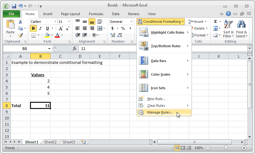
Conditional formatting in Excel allows you to automatically change the appearance of cells based on their values. This means you can highlight important data, identify trends, and quickly assess your information with just a few clicks. Whether you’re analyzing financial data, tracking project progress, or simply trying to organize your personal budget, conditional formatting can be an indispensable tool in your Excel arsenal.

Understanding Conditional Formatting

At its core, conditional formatting is all about defining rules. These rules specify how cell appearances should change based on specific criteria. Let’s break down the key components:

1. The Cell

This is the fundamental unit of your spreadsheet. You’re going to apply formatting rules to individual cells or a range of cells to change their appearance.

2. The Criteria

This is the heart of the conditional formatting process. It defines the specific conditions that must be met for the formatting to apply. You could use criteria based on:

• The Value of the Cell: Is the value greater than, less than, or equal to a specific number?
• The Text Contained in the Cell: Does the cell contain specific text, or does it begin or end with a certain word?
• The Cell’s Date: Is the date before, after, or equal to a specific date?
• A Formula: Does the result of a specific formula applied to the cell meet certain conditions?

Image: www.myxxgirl.com

3. The Formatting

This defines how the cell’s appearance will change when the criteria are met. You can modify:

• Font Color: Change the color of the text within the cell.
• Fill Color: Change the background color of the cell.
• Font Style: Make the text bold, italic, or underlined.
• Font Size: Increase or decrease the size of the text.
• Borders: Add or modify borders around the cell.
• Icons: Apply icon sets to visually represent data values.

Applying Conditional Formatting: A Step-by-Step Guide

Ready to put conditional formatting into action? Let’s walk through a practical example. Imagine you have a spreadsheet containing sales data for different products. You want to highlight the sales figures that are above a specific target, say 100 units sold.

1. Select the Range of Cells: Click and drag to select all the cells containing the sales figures you want to apply conditional formatting to.
2. Access the Conditional Formatting Menu: navigate to the “Home” tab in Excel and locate the “Conditional Formatting” group. Click on the “New Rule” button.
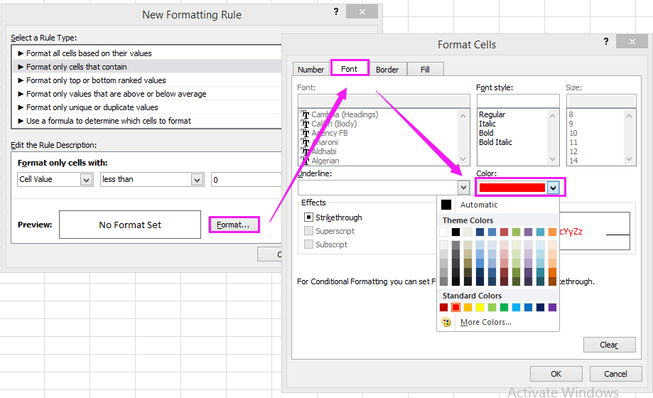
3. Choose a Rule Type: For our sales data example, we’ll use the “Format only cells that contain” rule type.
4. Define the Criteria: Select “Greater Than” from the dropdown menu. In the box next to it, enter the target value of 100 units.
5. Choose a Formatting Style: Click the “Format” button. You can now select a font color, fill color, or any other formatting options to apply to cells that meet the criteria. For instance, you might choose a green fill color to visually highlight the above-target sales values.
6. Apply the Formatting: Click “OK” to close the formatting window and “OK” again to apply the conditional formatting rule to your selected cells. Now, any sales figures exceeding 100 units will automatically be highlighted with the green fill color.

Beyond Basic Rules: Exploring Advanced Techniques

Conditional formatting isn’t just about applying basic rules to individual cells. Excel offers several advanced techniques to further enhance your data visualization:

1. Multiple Rules

You can apply multiple conditional formatting rules to the same range of cells. This allows you to create nuanced color-coding based on multiple criteria. For instance, in the sales data example, you could add a second rule to highlight sales figures lower than 50 units with a red fill color.

2. Data Bars

Data bars visually represent the values in cells as horizontal bars. Longer bars indicate larger values. This provides an immediate visual way to compare values within a range. Imagine applying data bars to your sales data – instantly you’d see which products have the highest sales.

3. Color Scales

Color scales apply a gradual color change to cells based on their values. This is useful for highlighting trends or identifying outliers. For instance, you could use a color scale to color-code your sales data, with lower sales values represented in blue and higher sales values in red.

4. Icon Sets

Icon sets apply small icons to cells based on defined values. These icons provide a quick visual indication of the value range for each cell. For example, you could use an icon set to represent sales figures: green arrows for sales exceeding the target, yellow arrows for values near the target, and red arrows for values below the target.

Real-World Applications of Conditional Formatting

Conditional formatting isn’t just a fancy visual tool; it has practical applications across various fields:

• Finance: Highlight financial statements that have significant variances from budget, identify potential risks, or analyze investment portfolio performance.
• Project Management: Track project progress, flag tasks that are overdue, or highlight critical milestones.
• Marketing: Analyze campaign performance, identify top-performing campaigns, and create visually compelling marketing reports.
• Sales: Identify top-performing sales reps, track sales targets, and monitor customer engagement.
• Education: Grade student assignments, pinpoint areas for improvement, and track academic progress.
• Personal Finance: Monitor your budget, identify spending patterns, and track investment returns.

Tips for Effective Conditional Formatting

To maximize the impact of conditional formatting, keep these tips in mind:

• Choose colors wisely: Select colors that contrast well with the background color of your spreadsheet and are visually clear. Avoid using colors that are too similar or that can be difficult to distinguish for colorblind users.
• Use clear criteria: Define your conditional formatting rules carefully so that the formatting accurately reflects the data you want to highlight.
• Test thoroughly: Apply your conditional formatting rules to a small sample of data first to ensure that the formatting works as expected.
• Maintain a consistent style: Try to use similar formatting styles throughout your spreadsheet to maintain consistency and visual coherence.
• Leverage pre-defined formatting styles: Excel includes a variety of pre-defined formatting styles that can save you time and ensure that your formatting is visually appealing.

Excel Change Color Of Cell Based On Value

Conclusion

Conditional formatting is a powerful tool that can transform your spreadsheets from static data tables into dynamic and insightful dashboards. By leveraging the ability to automatically change the appearance of cells based on their values, you can identify trends, highlight important data, and make your spreadsheets more visually appealing and informative. Start exploring the possibilities of conditional formatting today – your spreadsheets will thank you for it!