How to Change the Color of a Cell Based on Value – A Powerful Tool for Data Visualization

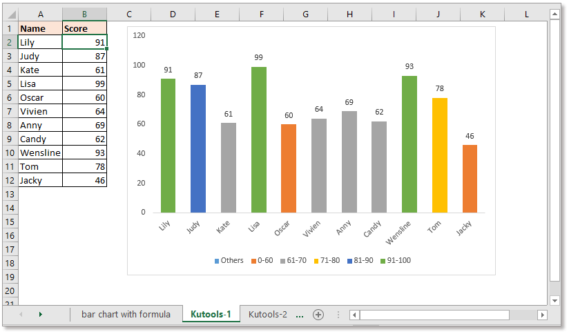
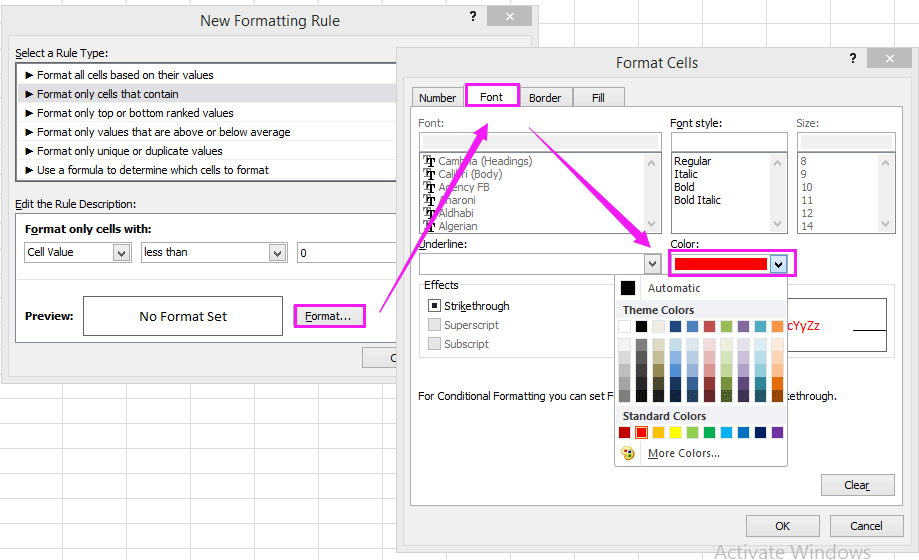
Imagine this: you have a spreadsheet filled with data, but it’s a sea of numbers and it’s tough to pull out the information you need. Wouldn’t it be great if you could instantly identify the highest values, the lowest ones, or any other important data points with just a glance? That’s where the ability to change cell colors based on values comes in. It’s a surprisingly effective tool that can transform your spreadsheets from bland data dumps to visually appealing and insightful dashboards.

Image: www.feevalue.com

In this article, we’ll explore the world of conditional formatting, a feature available in most spreadsheet software like Microsoft Excel, Google Sheets, and Apple Numbers. We’ll delve into the different ways you can use conditional formatting to color your cells, explore its various applications, and even show you some real-world examples of how it’s being used to analyze and present data more efficiently.

Why Change Cell Colors Based on Value?

You might be thinking, “Why bother changing the color of cells? Can’t I just filter or sort the data?” While filtering and sorting can be useful for specific tasks, conditional formatting offers distinct advantages that make it a powerful tool for data visualization and analysis:

1. Immediate Data Highlights:

Imagine you’re working with a sales spreadsheet and you need to quickly identify all the customers who have placed orders exceeding $1,000. Conditional formatting lets you instantly highlight those cells in a distinct color, allowing you to focus on the most important information without having to scroll through endless rows.

2. Visual Data Insights:

Conditional formatting is more than just highlighting; it provides a visual representation of your data. By using different color palettes, you can create heatmaps that show trends, variations, and patterns in your data. For example, you could use a range of colors to indicate sales performance, with green representing strong performance and red indicating areas needing improvement.

Image: woodlands.adventist.org

3. Dynamic Updates:

Conditional formatting rules are dynamic, meaning they automatically update as your data changes. If a customer’s order amount goes above the $1,000 threshold, the corresponding cell will instantly turn the designated color. This continuous update keeps your visual insights fresh and accurate in real-time.

Conditional Formatting Techniques:

Now that we understand the benefits of conditional formatting, let’s dive into the different ways you can change cell colors based on values. In most spreadsheet software, the core steps are similar, though specific features and options might vary:

1. Using Predefined Rule Sets:

This is the easiest way to get started. Most spreadsheet programs offer predefined rule sets for common tasks like highlighting the top ten values, highlighting duplicate values, or marking cells that are above or below a specific threshold.

• Example: To highlight the ten highest sales figures, simply select the cells containing the sales data, go to the “Conditional Formatting” menu, and choose the “Top 10 Items” rule. You can then customize the color and other formatting options.

2. Creating Custom Formatting Rules:

For more complex scenarios, you’ll need to create custom rules. This gives you complete control over how your cells are formatted based on specific conditions.

2.1. Using Formula-Based Rules:

You can use formulas to define conditions for cell formatting. This allows for highly flexible and tailored rules.

• Example: To change the cell color to green if a value is greater than 50 and red if the value is less than 20, you would create a formula-based rule with the formula: =A1>50 (for green) and =A1<20 (for red).

2.2. Using Icon Sets:

Icon sets allow you to represent values with icons in a more visual manner. For example, you can use three icons to represent low, medium, and high values.

• Example: You can set up a rule that places a green arrow icon next to sales values above a certain target, a yellow arrow for values near the target, and a red arrow for values below the target. This provides an instant visual indication of the performance level for each sales figure.

2.3. Using Data Bars:

Data bars are graphical representations of values within cells. They provide a visual comparison of values across a range of cells.

• Example: If you have a column of product sales figures, you can apply data bars to visually compare the sales volume of each product within the column. The longer the data bar, the higher the sales volume. This makes it easy to quickly identify the top-selling products.

2.4. Using Color Scales:

Color scales are another visual tool that uses color gradients to represent value ranges.

• Example: You could create a color gradient from green (low values) to red (high values) to represent the performance of different departments. This provides a visual overview of how each department is performing relative to the others.

Real-World Applications of Conditional Formatting:

The power of conditional formatting extends far beyond just making spreadsheets look prettier. Here are some real-world examples of how it can be used to analyze data and make informed decisions:

1. Sales Performance Analysis:

Sales teams can use conditional formatting to highlight top-performing salespersons, identify customers with high potential, or quickly analyze sales trends. By setting up rules based on sales targets, they can instantly visualize which team members are exceeding expectations, which are below target, and which areas need more focus.

2. Financial Analysis:

In finance, conditional formatting can help identify potential risks or opportunities by highlighting financial metrics that are outside of the expected range. This can be used to flag transactions that require further investigation, monitor cash flow, or identify companies with high or low financial ratios.

3. Project Management:

Project managers can use conditional formatting to track the progress of tasks, highlight overdue deadlines, or identify tasks that are at risk of falling behind schedule. By visually representing the status of tasks, it becomes easy to monitor project progress and take action when needed.

4. Quality Control:

In manufacturing or quality control, conditional formatting can be used to identify products that are outside of acceptable quality standards, monitor production line performance, or flag potential defects in a product. This helps streamline quality control processes and ensure that only compliant products are released to the market.

Adding a Touch of Color to Your Data:

Conditional formatting isn't just for serious applications; it can also be used to enhance the visual appeal and accessibility of your data presentations. You can use color gradients, subtle shading, and different color combinations to make your data more visually engaging. This can be particularly helpful for presentations, reports, and dashboards where clarity and aesthetics are crucial.

How To Change Color Of Cell Based On Value

Conclusion:

Changing the color of cells based on value isn't just about adding a splash of color to your spreadsheets; it's about transforming data into meaningful visual insights. Whether you are analyzing sales, tracking project progress, or simply making your data easier to digest, conditional formatting is a powerful tool that can unlock the full potential of your spreadsheets. Explore the different techniques, experiment with custom rules, and discover how this seemingly simple feature can significantly enhance your data visualization and analysis experience.